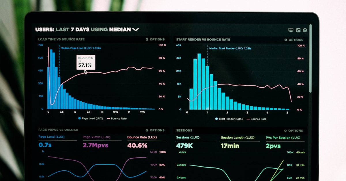
TimescaleDB Time Series Data Pipelines for IoT
TimescaleDB time series capabilities make it the ideal database for IoT data pipelines. As a PostgreSQL extension, TimescaleDB combines the reliability and ecosystem of PostgreSQL with specialized time-series optimizations — automatic partitioning, columnar compression, continuous aggregates, and data retention policies. This means your team can build high-performance IoT analytics without abandoning familiar SQL and PostgreSQL tooling. Because it is “just Postgres,” every driver, ORM, backup tool, and monitoring integration you already use continues to work, which is a decisive advantage over purpose-built time-series stores that force a new query language and operational model.
This guide covers building a complete IoT data pipeline from sensor ingestion to real-time dashboards. We will configure hypertables, implement compression policies, create continuous aggregates for fast analytics, and set up data retention for cost-effective long-term storage. Along the way we will dig into how chunking actually works, the gap-filling functions that make dashboards honest, and the trade-offs that determine whether TimescaleDB is the right call for your workload.
Architecture Overview
A typical IoT pipeline ingests thousands to millions of data points per second from sensors, stores them efficiently, and makes them queryable for real-time monitoring and historical analysis:
IoT Data Pipeline Architecture

Sensors/Devices → MQTT Broker → Ingestion Service → TimescaleDB
                                      ↓                  ↓
                              (batch inserts)    ┌────────────────┐
                                                 │ Hypertables    │
                                                 │ (raw data)     │
                                                 ├────────────────┤
                                                 │ Continuous     │
                                                 │ Aggregates     │
                                                 │ (1min, 1hr)    │
                                                 ├────────────────┤
                                                 │ Compression    │
                                                 │ (older data)   │
                                                 └────────────────┘
                                                        ↓
                                                 Grafana Dashboard
Setting Up TimescaleDB
-- Install TimescaleDB extension
CREATE EXTENSION IF NOT EXISTS timescaledb;

-- Create the sensor readings table
CREATE TABLE sensor_readings (
    time        TIMESTAMPTZ NOT NULL,
    device_id   TEXT NOT NULL,
    location    TEXT NOT NULL,
    temperature DOUBLE PRECISION,
    humidity    DOUBLE PRECISION,
    pressure    DOUBLE PRECISION,
    battery     DOUBLE PRECISION,
    metadata    JSONB DEFAULT '{}'
);

-- Convert to a hypertable (automatic time partitioning)
SELECT create_hypertable('sensor_readings', 'time',
    chunk_time_interval => INTERVAL '1 day',
    if_not_exists => TRUE
);

-- Add space partitioning for multi-tenant/multi-device
SELECT add_dimension('sensor_readings', 'device_id',
    number_partitions => 4
);

-- Create indexes for common query patterns
CREATE INDEX idx_readings_device_time
    ON sensor_readings (device_id, time DESC);
CREATE INDEX idx_readings_location
    ON sensor_readings (location, time DESC);
How Hypertables and Chunk Sizing Actually Work
A hypertable is a virtual table that TimescaleDB transparently splits into many physical child tables called chunks, each covering a slice of time. When you query the parent, the planner uses constraint exclusion to skip every chunk whose time range cannot match your WHERE clause — a technique called chunk pruning. Consequently, a query for the last hour touches one or two small chunks instead of scanning a multi-billion-row table, which is the core reason inserts and time-bounded reads stay fast as data grows.
Chunk sizing is the most important tuning knob, and the guidance is concrete rather than arbitrary. The docs recommend sizing chunks so that the most recent (uncompressed) chunks, together with their indexes, fit comfortably within roughly 25% of available memory. Chunks that are too large defeat pruning and bloat the cache; chunks that are too small create thousands of partitions whose planning overhead and metadata start to hurt. A daily interval suits a moderate-volume deployment, but a high-ingest fleet may want hourly chunks, while a low-volume historical archive might use weekly. You can change the interval at any time, and it only affects newly created chunks.
-- Inspect chunk sizes to validate your interval choice
SELECT chunk_name,
       range_start,
       range_end,
       pg_size_pretty(total_bytes) AS size
FROM chunks_detailed_size('sensor_readings')
ORDER BY range_start DESC
LIMIT 7;

-- Adjust the interval for future chunks (e.g. switch to hourly)
SELECT set_chunk_time_interval('sensor_readings', INTERVAL '1 hour');
High-Performance Data Ingestion
IoT pipelines require high write throughput. Moreover, batching inserts dramatically improves performance compared to individual row inserts:
import psycopg2
from psycopg2.extras import execute_values
import time
from collections import deque

class TimeseriesIngester:
    def __init__(self, dsn, batch_size=1000, flush_interval=5):
        self.conn = psycopg2.connect(dsn)
        self.conn.autocommit = False
        self.batch_size = batch_size
        self.flush_interval = flush_interval
        self.buffer = deque()
        self.last_flush = time.time()

    def insert(self, reading):
        """Buffer a reading for batch insert."""
        self.buffer.append((
            reading['time'],
            reading['device_id'],
            reading['location'],
            reading['temperature'],
            reading['humidity'],
            reading['pressure'],
            reading['battery'],
        ))

        if (len(self.buffer) >= self.batch_size or
                time.time() - self.last_flush > self.flush_interval):
            self.flush()

    def flush(self):
        """Batch insert buffered readings."""
        if not self.buffer:
            return

        batch = list(self.buffer)
        self.buffer.clear()

        with self.conn.cursor() as cur:
            execute_values(
                cur,
                """INSERT INTO sensor_readings
                   (time, device_id, location, temperature,
                    humidity, pressure, battery)
                   VALUES %s""",
                batch,
                page_size=self.batch_size
            )
        self.conn.commit()
        self.last_flush = time.time()
        print(f"Flushed {len(batch)} readings")

# Usage: a single batched writer handles tens of thousands of inserts/second
ingester = TimeseriesIngester(
    'postgresql://user:pass@localhost/iot',
    batch_size=5000,
    flush_interval=2
)
Late-Arriving Data and Idempotent Ingestion
The tidy diagram above hides a messy reality: IoT data does not arrive in order. Devices buffer readings while offline, mobile gateways reconnect after hours in a tunnel, and clock drift means timestamps wander. A robust pipeline must therefore handle out-of-order and duplicate readings gracefully. TimescaleDB happily accepts inserts into older chunks, but if that data falls inside a window a continuous aggregate has already materialized, you need the aggregate’s invalidation tracking to refresh it — which is why the refresh policy below intentionally reaches back several hours rather than only covering the present moment.
Duplicates are the other hazard, since a retrying gateway may resend a batch it already delivered. Adding a unique constraint on the device and timestamp, combined with an upsert, makes ingestion idempotent so retries cannot inflate your counts. This single change turns a fragile pipeline into one that tolerates network flakiness without manual cleanup.
-- Make (device_id, time) unique so retries don't double-count
ALTER TABLE sensor_readings
    ADD CONSTRAINT uq_device_time UNIQUE (device_id, time);

-- Idempotent batch insert: ignore exact replays
INSERT INTO sensor_readings (time, device_id, location, temperature, humidity)
VALUES ('2026-06-12 10:00:00+00', 'dev-42', 'plant-a', 21.4, 55.2)
ON CONFLICT (device_id, time) DO NOTHING;
Continuous Aggregates for Fast Analytics
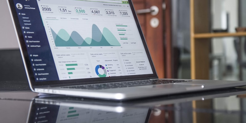
Continuous aggregates automatically pre-compute time-bucketed summaries. Therefore, dashboard queries that would scan millions of rows instead read pre-materialized results:
-- 1-minute aggregates (real-time materialized view)
CREATE MATERIALIZED VIEW sensor_readings_1min
WITH (timescaledb.continuous) AS
SELECT
    time_bucket('1 minute', time) AS bucket,
    device_id,
    location,
    AVG(temperature) AS avg_temp,
    MIN(temperature) AS min_temp,
    MAX(temperature) AS max_temp,
    AVG(humidity) AS avg_humidity,
    AVG(pressure) AS avg_pressure,
    AVG(battery) AS avg_battery,
    COUNT(*) AS reading_count
FROM sensor_readings
GROUP BY bucket, device_id, location
WITH NO DATA;

-- Refresh policy: auto-update aggregates
SELECT add_continuous_aggregate_policy('sensor_readings_1min',
    start_offset => INTERVAL '3 hours',
    end_offset => INTERVAL '1 minute',
    schedule_interval => INTERVAL '1 minute'
);

-- 1-hour aggregates (for historical dashboards)
CREATE MATERIALIZED VIEW sensor_readings_1hr
WITH (timescaledb.continuous) AS
SELECT
    time_bucket('1 hour', bucket) AS bucket,
    device_id,
    location,
    AVG(avg_temp) AS avg_temp,
    MIN(min_temp) AS min_temp,
    MAX(max_temp) AS max_temp,
    AVG(avg_humidity) AS avg_humidity,
    SUM(reading_count) AS reading_count
FROM sensor_readings_1min
GROUP BY time_bucket('1 hour', bucket), device_id, location
WITH NO DATA;

SELECT add_continuous_aggregate_policy('sensor_readings_1hr',
    start_offset => INTERVAL '2 days',
    end_offset => INTERVAL '1 hour',
    schedule_interval => INTERVAL '1 hour'
);
Gap Filling and Last-Observation Dashboards
Raw sensor data has holes — a device drops offline, a packet is lost, and a bucket ends up with no rows. A naive dashboard then draws a misleading line straight across the missing interval, or worse, omits the gap entirely so a flat-lining sensor looks healthy. TimescaleDB’s time_bucket_gapfill function solves this honestly by emitting a row for every interval in the requested range, even empty ones, and then offering interpolation or last-observation-carried-forward to fill them deliberately rather than by accident.
-- Continuous, gap-free series for a Grafana panel
SELECT
    time_bucket_gapfill('5 minutes', time) AS bucket,
    device_id,
    avg(temperature)              AS avg_temp,
    locf(avg(temperature))        AS temp_last_known,  -- carry forward
    interpolate(avg(temperature)) AS temp_interpolated -- linear fill
FROM sensor_readings
WHERE time > now() - INTERVAL '6 hours'
  AND device_id = 'dev-42'
GROUP BY bucket, device_id
ORDER BY bucket;
Choosing between locf and interpolate is a real modeling decision. For a slowly changing value like a thermostat setpoint, carrying the last known value forward is correct; for a smoothly varying physical signal, linear interpolation reads better. Either way, the explicit gap is the point — surfacing missing data is what separates a trustworthy monitoring dashboard from one that quietly hides outages.
Compression and Data Retention
TimescaleDB columnar compression reduces storage by 90-95%. Additionally, retention policies automatically drop old data to manage costs:
-- Enable compression on the hypertable
ALTER TABLE sensor_readings SET (
    timescaledb.compress,
    timescaledb.compress_segmentby = 'device_id',
    timescaledb.compress_orderby = 'time DESC'
);

-- Auto-compress data older than 7 days
SELECT add_compression_policy('sensor_readings',
    compress_after => INTERVAL '7 days'
);

-- Retention: drop raw data older than 90 days
SELECT add_retention_policy('sensor_readings',
    drop_after => INTERVAL '90 days'
);

-- Keep 1-min aggregates for 1 year
SELECT add_retention_policy('sensor_readings_1min',
    drop_after => INTERVAL '1 year'
);

-- Keep hourly aggregates forever (no policy)

-- Check compression stats
SELECT
    pg_size_pretty(before_compression_total_bytes) AS before,
    pg_size_pretty(after_compression_total_bytes) AS after,
    round((1 - after_compression_total_bytes::numeric /
           before_compression_total_bytes) * 100, 1) AS ratio
FROM hypertable_compression_stats('sensor_readings');
The Hidden Cost of Compression: segmentby and Mutability
Compression delivers dramatic savings, but it changes how a chunk behaves, and the compress_segmentby choice drives whether those savings materialize. Segmenting by device_id groups all rows for a device together and stores each metric column as a contiguous, type-aware array, which compresses far better than a row store and lets queries filtered by that device skip irrelevant segments entirely. Choose the wrong segment key — something high-cardinality and rarely filtered on — and you sacrifice both ratio and query speed. As a rule, segment by the column you most often filter on, and order by time.
The trade-off worth internalizing is mutability. Compressed chunks were historically read-mostly: modern TimescaleDB does support updates and deletes against them, but those operations are slower than on uncompressed data and may decompress segments behind the scenes. Therefore the cleanest pattern is to compress only chunks old enough that they are effectively immutable, which is exactly why the policy above waits seven days. If your workload genuinely rewrites week-old readings, push the compression threshold further out rather than fighting the engine.
When NOT to Use TimescaleDB
TimescaleDB is optimized for time-series workloads. If your data is not time-ordered — for example, a social network graph, product catalog, or document store — PostgreSQL without TimescaleDB is more appropriate. Furthermore, for extremely high cardinality metrics (millions of unique series), dedicated metrics databases like VictoriaMetrics or Mimir may be more efficient. If you need global multi-region replication with strong consistency, managed solutions like Amazon Timestream might be simpler to operate.
There are subtler boundaries too. If your analytics are purely historical and never need updates or transactions — terabytes of immutable events scanned for ad-hoc OLAP — a columnar engine such as ClickHouse or DuckDB will likely outrun TimescaleDB on wide aggregate scans, a comparison explored in our analytical databases write-up. Conversely, the moment you need joins to relational reference data, ACID transactions, row-level updates, or the broad PostgreSQL extension ecosystem alongside your time-series tables, TimescaleDB’s “it’s just Postgres” nature becomes the deciding advantage. The honest framing is that TimescaleDB occupies the sweet spot where you want strong time-series performance without giving up SQL, relational integrity, and operational familiarity — and it is the wrong tool when you can give those up for raw scan throughput, or when your data was never temporal to begin with.

Key Takeaways
- TimescaleDB time series capabilities extend PostgreSQL with automatic partitioning, compression, and continuous aggregates
- Size chunks so recent ones fit in memory, and make ingestion idempotent to survive retries and out-of-order data
- Continuous aggregates pre-compute time-bucketed summaries, reducing dashboard query times from seconds to milliseconds
- Use gap filling with locf or interpolate so dashboards surface missing data honestly instead of hiding outages
- Columnar compression with a well-chosen segmentby key reduces storage by 90-95% for effectively immutable older data
Related Reading
External Resources
In conclusion, Timescaledb Iot Time Series is an essential topic for modern software development. By applying the patterns and practices covered in this guide — right-sized chunks, idempotent batched ingestion, gap-filled continuous aggregates, and tiered compression with retention — you can build more robust, scalable, and maintainable systems. Start with the fundamentals, iterate on your implementation, and continuously measure results to ensure you are getting the most value from these approaches.